This paper introduces an advanced approach to analysing atmospheric turbulence in subcarrier quadrature amplitude modulation (SC-QAM) free space optical (FSO) systems through a development and application of the exponentiated gamma channel model. The study focuses on FSO systems with multiple receivers, employing Greedy scheduling to optimize link performance. A closed-form expression for the average bit error rate (BER) is derived, leveraging the SC-QAM modulation technique and the exponentiated gamma channel model to characterise turbulence-induced fading accurately. To enhance system robustness, the use of multiple receivers is proposed, and a novel expression for the BER in a multiple-output configuration is developed. Comprehensive simulations are conducted to validate the accuracy of the derived closed-form BER expression and to investigate the influence of key system parameters on performance. The analysis examines factors such as the link distance and the refractive index structure parameter, which are critical in determining the impact of turbulence on FSO links. The results demonstrate the significant benefits of employing multiple receivers, with Greedy scheduling shown to play a pivotal role in mitigating turbulence effects and improving overall BER performance. Furthermore, the findings highlight that increasing the number of receivers substantially enhances the system resilience to fading and turbulence, leading to a robust reduction in BER. This study not only provides valuable insights into the optimization of FSO systems under turbulence but also establishes a framework for future research on advanced scheduling algorithms and modulation techniques. The results underscore the importance of system design parameters and provide practical recommendations for enhancing the reliability and efficiency of the next-generation FSO communication networks.

Introduction

Free space optical (FSO) communication has emerged as a compelling alternative in modern telecommunication due to its inherent advantages, including high-speed data transmission, use of unlicensed spectrum, and cost-effective deployment. Its applicability spans a broad spectrum of use cases, ranging from last-mile connectivity and inter-building links to satellite communication and autonomous system integration. Despite these promising characteristics, FSO systems are highly vulnerable to atmospheric conditions, with turbulence posing a particu-larly significant challenge. Caused by spatial and temporal variations in temperature, pressure, and humidity, atmospheric turbulence induces random fluctuations in the refractive index, which in turn severely degrade the integrity of the transmitted optical signals. These effects are typically modelled using statistical channel distributions, which depend on parameters such as turbulence regime, link distance, and the refractive index structure constant.

To counteract the impact of turbulence, techniques such as receiver diversity and deployment of multiple receivers have been extensively explored. Several statistical models have been proposed to characterise the fading effects induced by atmospheric turbulence under varying condi-tions. The log-normal model is widely used for modelling weak turbulence due to its mathematical simplicity and reasonable accuracy. However, it suffers from inherent limitations, particularly its tendency to underestimate both the peak and the tails of the probability density function (PDF), which can result in suboptimal system performance predictions [1, 2]. For scenarios involving strong turbu-lence, the K-distribution model is often preferred as it offers lower outage probabilities with increasing diversity order and wavelength. However, its inability to effectively model weak turbulence restricts its broader applicability. In combination with the I-distribution, the model becomes more versatile, capable of handling both weak and strong turbulence conditions more effectively [3, 4].

The gamma-gamma distribution has gained prominence due to its ability to capture both small-scale and large-scale irradiance fluctuations, making it suitable for a wide range of turbulence levels. Its effectiveness is bolstered by its strong alignment with empirical data and simulation outcomes. System performance under gamma-gamma conditions can be further enhanced by using robust modu-lation schemes, such as subcarrier intensity modulation (SIM) [5]. For extended link distances, typically spanning several kilometres, the negative exponential distribution has been favoured. This model is particularly suitable for environments with strong turbulence, offering advantages in terms of channel capacity and bit error rate (BER) reduction [6].

Alternative models such as the I-G distribution have shown promise under weak turbulence conditions but tend to exhibit extended fade durations at higher operating wavelengths [7]. The Weibull distribution is effective in representing both small- and large-scale fading. Its enhanced variant, the double Weibull distribution provides a more accurate depiction under moderate turbulence by closely matching observed experimental data [8]. More recently, the double generalized gamma distribution has demonstrated an improved accuracy across a broad spectrum of turbulence intensities, outperforming both the double Weibull and gamma-gamma models in simulation comparisons, thus positioning itself as a highly adaptable channel model [9].

On the system configuration front, a single-input multiple-output (SIMO) FSO systems have been shown to yield significant improvements in communication reliability and BER performance. For instance, SIMO FSO systems employing a maximum ratio combining (MRC) with log-normal turbulence and differential phase shift keying (DPSK) have demonstrated enhanced BER outcomes. Notably, a binary phase shift keying (BPSK) has outperformed DPSK under similar conditions, particularly when integrated with MRC. Additional enhancements such as aperture averaging and optimized receiver combining techniques have further improved resilience against turbulence-induced degradations. These improvements are particularly critical under strong turbulence conditions, where the performance degradation is more severe compared to moderate or weak turbulence regimes.

FSO communication systems have shown considerable promise in various applications, including last-mile connectivity, satellite communication, and autonomous systems. FSO offers high-speed data transfer capabilities that rival fibre optic communication, making it a viable alternative for urban broadband deployment where laying fibre is impractical [10]. Additionally, FSO systems operate in the unlicensed optical spectrum, offering a significant advantage in terms of regulatory flexibility compared to radio frequency (RF) systems. The technology is also cost-effective, with relatively low-cost components such as lasers and photodetectors, making it an attractive option for both urban and remote area deployments [11]. Furthermore, FSO high bandwidth capabilities and suitability for use in autonomous systems, including drones, position it as a strong candidate for future communication networks, especially in satellite and inter-satellite links [12, 13].

The integration of FSO with complementary communication technologies presents a fertile avenue for research. Hybrid architectures that combine FSO with RF or optical fibre networks could offer robustness against visibility fluctuations and environmental disruptions. However, optimizing such hybrid systems – particularly with respect to dynamic link switching, load balancing, and joint resource management – remains an open challenge requiring further investigation.

While the relationship between signal-to-noise ratio (SNR) and BER has been extensively studied and well-established in the context of optical wireless communi-cation, much of the existing literature focuses on traditional turbulence models such as log-normal, gamma-gamma, and K-distributions [1–5]. These models provide analytical expressions for BER performance under varying turbulence regimes using classical mathematical tools. However, most studies reiterate standard SNR-BER expressions without introducing substantial novelty, particularly in terms of channel adaptability or real-time scheduling. In contrast, the present work aims to build upon these foundational principles by integrating the exponentiated gamma channel model capable of characterising a wider range of turbulence conditions with a subcarrier quadrature amplitude modulation (SC-QAM) modulation and Greedy scheduling. This combination enables a more flexible and performance-optimized approach to FSO system design, especially under dynamic and heterogeneous atmospheric conditions. Recognizing these challenges, the current paper introduces a sophisticated FSO system that incorporates multiple outputs, Greedy scheduling, and exponentiated gamma turbulence model in conjunction with SC-QAM. This integrated approach not only aims to improve BER performance in turbulence-prone environments but also addresses some of the most pressing limitations found in existing models. By exploring this enhanced configuration, the study makes a significant contribution to the develop-ment of robust and efficient optical wireless communication systems.

SISO FSO system with SC-QAM

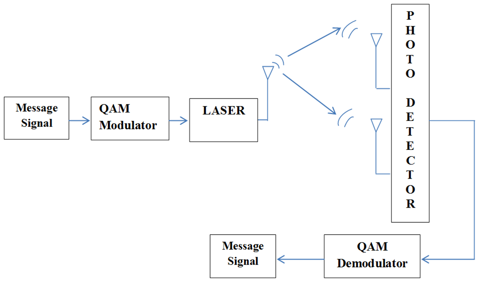
Fig. 1 illustrates the block diagram of a single-input single-output (SISO) FSO system. The system comprises a single transmitter and multiple spatially separated receivers.

Fig. 1. Block diagram of the SISO FSO system.

The input message signal is first encoded using quadrature amplitude modulation (QAM), a modulation scheme known for its high spectral efficiency. The modulated signal is then used to drive an optical modulator, converting the electrical QAM signal into an optical signal suitable for free space transmission. The input message signal is converted into a QAM signal and is expressed as:

where Q_Q(t) and Q_I(t) represent the quadrature and the in-phase signals, respectively. The QAM signal is optically modulated using an optical modulator. It is transmitted from the transmitter section and is given as:

where x(t) is the carrier signal and q(t) is the QAM signal. The transmitted optical signal is received by the receiver and is given as an input to a photo detector, which converts optical signal into electrical signal [14].

\( y(t)=A S x(t)(1+q(t))\left(1+k\left(Q_I(t) \cos 2 \pi f_x t-Q_Q(t) \sin 2 \pi f_x t\right)\right), \) (4)

where k represents the modulation index, A indicates the attenuation, and S represents the scintillation.

\( \begin{aligned} y_{p d}(t) & =A S x(t)(1+q(t)) \\ & R k\left(Q_I(t) \cos 2 \pi f_x t-Q_Q(t) \sin 2 \pi f_x t\right)+f(t) \end{aligned} \) (5)

The signal represented by (5) is demodulated by the QAM demodulator and generates an original message signal.

PDF of hybrid channel model

This section presents the PDF of a hybrid channel model, which is a combination of exponential model and gamma channel model. Initially, a model based on gamma distribution is derived. This model is extended into the exponentiated gamma channel model for FSO system.

Gamma fading

Many distributions have been presented to find PDF for describing irradiance fluctuation in FSO system [5]. Assume that fluctuation takes place due to the modulation between large and small scale irradiance, i.e.: irradiance I = P where P is the random variable.

where P1, P2, …, Pm are the variates and the irradiance Pi follows a negative exponential distribution. The random variable P terms of its characteristic function [15] is:

\( \varphi_P(w)=\left[\frac{1}{1-j w\left\langle P_i\right\rangle}\right]^m \) (8)

The PDF of gamma distribution can be obtained by applying an inverse Fourier transform (IFT) for characteristics function:

\( f_P(P)=F^{-1}\left\{\left[\frac{1}{1-j w\left\langle P_i\right\rangle}\right]^m\right\} \) (9)

\( f_P(P)=\frac{1}{\left\langle P_i\right\rangle^m(m-1)!} P^{m-1} e^{-P /\left(P_i\right)} \) (10)

\( f_P(P)=\frac{\alpha(\alpha P)^{\alpha-1}}{\Gamma(\alpha)} \exp (-\alpha P) \) (11)

Expressing α in terms of scintillation index, equations (11) and (12) can be expressed as:

\( f_P(P)=\frac{(P)^{\alpha-1}}{i \Gamma(\alpha) \sigma_i^2} \exp \left(-P / \sigma_i^2\right) \) (13)

\( f_I(I)=\frac{(P)^{\alpha-1}(Q)^{\beta-1}}{i j \Gamma(\alpha) \sigma_i^2} \exp \left\{\left(\frac{-P}{\sigma_i^2}\right)+\left(\frac{-Q}{\sigma_j^2}\right)\right\} \) (15)

\( f_I(I)=\int_0^{\infty} f_{I_p}\left(I / I_Q\right) \cdot f_{I_Q}\left(I_Q\right) d I_Q \) (16)

\( \begin{aligned} & f_I(I)= \\ & \int_0^{\infty}\left(\frac{\left(\frac{I}{I_Q}\right)^{\alpha-1}}{i \Gamma(\alpha) \sigma_i^2} \exp \left(-\left(\frac{I}{I_Q}\right) \frac{1}{\sigma_i^2}\right)\right) \cdot\left(\frac{\left(I_Q\right)^{\beta-1}}{j} \exp \left(-\left(\frac{I}{I_Q}\right) 1 / \sigma_j^2\right) d I_Q\right. \end{aligned} \) (17)

Using Meijer’s G-function (MGF) [16], the above expression can be simplified as:

\( \begin{array}{r} f_I(I)=\frac{q^{\alpha-1}}{\Gamma(\alpha)} q^{\alpha-1} \cdot I^{-1} G_{p+q .0}^{0, p+q}\left[\left.\sigma_i^2 q^\alpha \sigma_j^2 p^\beta \cdot \frac{\sigma_j^\beta}{I_v^{\beta-1}} \right\rvert\,\right. \\ \Delta(q: 1-\alpha), \Delta(p \cdot 1-\beta) . \end{array} \) (18)

BER of exponentiated gamma channel model

This section presents the BER of the exponentiated gamma channel model. Under atmospheric turbulence, the error probability is expressed as:

\( P_e=\frac{1}{2} \int_0^{\infty} \operatorname{erfc}\left(\frac{\mathrm{SNRI}}{2 \sqrt{2}}\right) f_I(I) d I \) (19)

Here erfc(.) is the complementary error function. Expressing erfc(.) as MGF [17], the above expression can be rewritten as:

\( P_b=\frac{1}{2 \sqrt{\pi}} \int_0^{\infty} G_{1,2}^{2,0}\left[\left\{\left.\frac{(\mathrm{SNRI})^2}{8} \right\rvert\, 0, \frac{1}{2}\right\} f_I(I) d I\right] \) (20)

Based on above expression, the closed-form expression for BER of the exponentiated gamma channel is derived. That is:

\( \begin{aligned} P_b= & \frac{1}{2 \sqrt{\pi}} \int_0^{\infty} G_{1,2}^{2,0}\left[\left\{\frac{(\mathrm{SNRI})^2}{8} \left\lvert\, \begin{array}{c} 1 \\ 0, \frac{1}{2} \end{array}\right.\right\}\right] \\ & \left\{\begin{array}{l} \frac{q^{\alpha-1}}{\Gamma(\alpha)} q^{\alpha-1} \cdot I^{-1} G_{p+q, 0}^{0, p+q} \\ {\left[\left.\sigma_i^2 q^\alpha \sigma_j^2 p^\beta \cdot \frac{\sigma_j^\beta}{I_v^{\beta-1}} \right\rvert\, \Delta(q: 1-\alpha), \Delta(p .1-\beta)\right.} \end{array}\right\} d I . \end{aligned} \) (21)

\( \left.\begin{array}{rl} P_b & =\frac{1}{2 \sqrt{\pi}} G_{1,3}^{2,1}\left(\left.\frac{\mathrm{SNRI}^2}{8}\right|_{\frac{1,3}{2}} ^2\right) \\ & \left\{\begin{array}{l} \frac{q}{\Gamma(\alpha)} q \cdot I^{-1} G_{p+q+1,1}^{0, p+q+1} \times \\ \left(\left.\sigma_i^2 q^\alpha \sigma_j^2 p^\beta \cdot \frac{\sigma_j^\beta}{I_v^{\beta-1}} \right\rvert\, \Delta(\alpha+q, \alpha+1),\right. \\ \Delta(\alpha+p) \end{array}\right) \end{array}\right\} \) (22)

Above expression gives the simplified form of BER of the exponentiated gamma channel model.

BER of SIM-QAM exponentiated gamma channel model

This section presents BER of SIM-QAM with the exponentiated gamma channel model in the presence of atmospheric turbulence. BER of the QAM signal can be obtained from BER of two-pulse amplitude modulation (PAM) signals [18].

\( P_{\frac{I}{\gamma}}(k)=\frac{1}{I} \sum_{i=0}^{\left(1-2^{-k}\right) I-1}\left\{\begin{array}{l} \left.(-1)^{\frac{i \cdot 2^{k-1}}{I}}\right] \times\left(2^{k-1}-\left[\frac{i \cdot 2^{k-1}}{I}+\frac{1}{2}\right]\right) \times \\ \operatorname{erfc}\left((2 i+1)-\sqrt{\frac{3 \log _2(I \cdot J) \gamma}{I^2+J^2-2}}\right) \end{array}\right\} \) (23)

\( P_{\frac{J}{\gamma}}(l)=\frac{1}{J} \sum_{j=0}^{\left(1-2^{-1}\right)^{J^{-1}}}\left\{\begin{array}{l} (-1)^{\frac{j \cdot 2^{l-1}}{J}} \times\left(2^{I-1}-\left[\frac{i \cdot 2^{I-1}}{J}+\frac{1}{2}\right]\right) \times \\ \operatorname{erfc}\left((2 j+1)-\sqrt{\frac{3 \log _2(I \cdot J) \gamma}{I^2+J^2-2}}\right) \end{array}\right\} \) (24)

where P_I/y(k) and P_j/y(l) are the conditional kth and lth BER, respectively. γ indicates the SNR and erfc(.) is the complementary function [19]. The average of kth and lth BER is given as:

\( P_I(k)=\int_{\gamma=0}^{\infty} P_{I / \gamma}(k) f_\gamma(\gamma) d \gamma \) (25)

\( P_I(k)=\frac{1}{I} \sum_{i=0}^{\left(1-2^{-k}\right) I-1}\left\{\begin{array}{l} \left.(-1)^{\left[\frac{i-2^{k-1}}{I}\right.}\right]_{\times} \\ \left(2^{k-1}-\left[\frac{i \cdot 2^{k-1}}{I}+\frac{1}{2}\right]\right) \times \\ \int_0^{\infty} \operatorname{erfc}\left((2 i+1) \sqrt{\frac{3 \log _2(I \cdot J) \gamma}{I^2+J^2-2}}\right) \\ \left.\left.\left\{\begin{array}{l} \frac{(P / \gamma)^{\alpha-1}(\gamma)^{\beta-1}}{i j \Gamma(\alpha) \sigma_i^2} G_{0,1}^{1,0} \\ \left\{\left(\frac{-\left(\frac{P}{\gamma}\right)}{\sigma_i^2}\right)+\binom{-(Q / \gamma)}{\sigma_j^2}\right) \end{array}\right\}\right]\right\} d \gamma \end{array}\right\}, \) (26)

where f_γ(γ) is obtained by expressing (15) in terms of MGF and after applying power transformation of fI(I). By expressing erfc(.) in terms of MGF, the above equation can be expressed as:

\( \begin{aligned} & P_I(k)= \\ & \frac{1}{I} \sum_{i=0}^{\left(1-2^{-k}\right) I-1}\left\{\begin{array}{l} (-1)^{\left[\frac{i 2^{k-1}}{I}\right]} \times \\ \left(2^{k-1}-\left[\frac{i \cdot 2^{k-1}}{I}+\frac{1}{2}\right]\right) \times \\ \frac{1}{\sqrt{\pi}} G_{1,2}^{2,0}\left(\left.\frac{(2 i+1)^2 3 \log _2(I \cdot J) \gamma}{I^2+J^2-2}\right|_{0, \frac{1}{2}} ^1\right. \\ \left\{\begin{array}{l} \left.\frac{(P / \gamma)^{\alpha-1}(\gamma)^{\beta-1}}{i j \Gamma(\alpha) \sigma_i^2} G_{0,1}^{1,0}\left[\binom{-\left(\frac{P}{\gamma}\right)}{\sigma_i^2}+\left\lvert\, \begin{array}{l} - \\ 0 \\ \left.\left(\frac{-(Q / \gamma)}{\sigma_j^2}\right) \right\rvert\, \end{array}\right.\right)\right] \end{array}\right\} \end{array}\right\} \end{aligned} \) (27)

\( \begin{aligned} & P_I(l)= \\ & \frac{1}{J} \sum_{i=0}^{\left(1-2^{-l}\right) J-1}\left\{\begin{array}{l} (-1)^{\left[\frac{i \cdot 2^{l-1}}{J}\right]} \times \\ \left(2^{i-1}-\left[\frac{j \cdot 2^{l-1}}{J}+\frac{1}{2}\right]\right) \times \\ \frac{1}{\sqrt{\pi}} G_{1,2}^{2,0}\left(\left.\frac{(2 j+1)^2 3 \log _2(I . J) \gamma}{I^2+J^2-2}\right|_{0, \frac{1}{2}} ^1\right. \\ \left.\left\{\begin{array}{l} \frac{(P / \gamma)^{\alpha-1}(\gamma)^{\beta-1}}{i j \Gamma(\alpha) \sigma_i^2} G_{0.1}^{1,0}\left(\left[\begin{array}{l} \left(\frac{-\left(\frac{P}{\gamma}\right)}{\sigma_i^2}\right) \\ \left(\frac{-(Q / \gamma)}{\sigma_j^2}\right) \end{array}\right)\right] \end{array}\right\}\right] \end{array}\right\} \end{aligned} \) (28)

\( P_b=\frac{1}{\log _2(I \cdot J)}\left(\sum_{k=1}^{\log _2 I} P_I(k)+\sum_{i=1}^{\log _2 J} P_J(l)\right) \) (29)

Substituting (27) and (28) in (29) gives BER of the rectangular QAM signal with the exponentiated gamma channel model. If I = J =M, (29) becomes

\( P_b(k)=\frac{1}{\sqrt{M}} \sum_{i=0}^{\left(1-2^{-k}\right) \sqrt{M-1}}\left\{\begin{array}{l} (-1)^{\left.\frac{\left[1-2^{k-1}\right.}{\sqrt{M}}\right]} \times\left(2^{k-1}-\left[\frac{i \cdot 2^{k-1}}{\sqrt{M}}+\frac{1}{2}\right]\right) \times \\ \frac{1}{\sqrt{\pi}} G_{1,2}^{2,0}\left(\left.\frac{(2 \sqrt{M}+1)^2 3 \log _2(M) \gamma}{2(M-1)}\right|_{0, \frac{1}{2}} ^1\right) \times \\ \left.\left[\begin{array}{l} \frac{(P / \gamma)^{\alpha-1}(\gamma)^{\beta-1}}{i j \Gamma(\alpha) \sigma_{\mathrm{i}}^2} G_{0,1}^{1,0} \\ {\left[\left\{\left(\frac{-(P / \gamma)}{\sigma_{\mathrm{i}}^2}\right)+\left.\left(\frac{-(Q / \gamma)}{\sigma_{\mathrm{j}}^2}\right)\right|^{-}\right]\right.} \\ 0 \end{array}\right]\right] \end{array}\right\} . \) (31)

Substitution of (31) in (30) gives BER of a M-ary quadrature amplitude modulation (M-QAM):

\( \sum_{k=1}^{\sqrt{M}} \frac{1}{\sqrt{M}} \sum_{i=0}^{\left(1-2^{-k}\right) \sqrt{M}-1}\left\{\begin{array}{l} (-1)^{\left[\frac{i-2^{k-1}}{\sqrt{M}}\right]} \times\left(2^{k-1}-\left[\frac{i \cdot 2^{k-1}}{\sqrt{M}}+\frac{1}{2}\right]\right) \times \\ \frac{1}{\sqrt{\pi}} G_{1,2}^{2,0}\left(\left.\frac{(2 \sqrt{M}+1)^2 3 \log _2(M) \gamma}{2(M-1)}\right|_{0, \frac{1}{2}} ^1\right) \times \\ \left.\left\{\begin{array}{l} \frac{(P / \gamma)^{\alpha-1}(\gamma)^{\beta-1}}{i j \Gamma(\alpha) \sigma_{\mathrm{i}}^2} \\ G_{0,1}^{1,0}\left[\left\{\left.\left(\frac{-(P / \gamma)}{\sigma_{\mathrm{i}}^2}\right)+\left(\frac{-(Q / \gamma)}{\sigma_{\mathrm{j}}^2}\right) \right\rvert\,-1\right]\right. \\ 0 \end{array}\right\}\right] \end{array}\right\} \) (32)

Above expression represents the average BER of the M-QAM exponentiated gamma channel model

SIMO-FSO system with exponentiated gamma channel model and Greedy scheduling

SIMO FSO system consists of a single transmitter and a multiple receiver. Consider a node which consists of N transmit apertures in which ith transmit aperture is sending data to the ith receiver aperture as shown in Fig. 1. The transmit aperture is selected based on time division multiplexing manner, i.e., a particular transmit aperture remains active in a particular time slot [20]. As in SISO system, the input signal is modulated using QAM, which is followed by optical modulation. If a channel model describes weak turbulence, light propagation occurs under clear weather condition, during which the effect of absorption gets vanished [21]. The exponentiated gamma channel model describes all types of turbulence such as weak, moderate, and strong. PDF of the exponentiated gamma channel model is:

\( f_I(I)=\frac{(P)^{\alpha-1}(Q)^{\beta-1}}{i j \Gamma(\alpha) \sigma_i^2} \exp \left\{\left(\frac{-P}{\sigma_i^2}\right)+\left(\frac{-Q}{\sigma_j^2}\right)\right\} \) (33)

P and Q indicate the irradiance, σ_i² = σ_j² = σ_R² indicates the Rytov variance, α and β are the parameters of gamma and exponential function.

SIMO transfers data to the user based on the condition of the channel. Diversity gain of such system is mainly influenced by the turbulence strength which is defined by the Rytov variance. Consider the SIMO system and assume that the user at the output sends its state information to the node at the transmit end. After receiving state information, the link rate is given as:

Where ,ninγ is the SNR for a given time slot. The important purpose of scheduling is to accomplish the maximum throughput and the minimum latency. The central node identifies the best user based on the channel state information (CSI) and is expressed as:

\( i_n^*=\arg \underbrace{\max }_{1 \mathrm{~s} \pi \leqslant N} \frac{R_{i_n, n}}{\bar{R}_{i_n, n}}, \) (35)

\( \bar{R}_{t_n, n}=\frac{\log \left(1+\left(\left(\left(\mathrm{alpa}^2\right) *\left(f_I(I)^2\right) *\left(\mathrm{p} / N_o\right)\right) \cdot(\mathrm{p}-1)\right)\right)}{p_{\max }} \) (36)

p/No is the fixed parameter, pmax represents the maximum number of users, fI(I) is the PDF of the exponentiated gamma channel, and li is the distance between the central node and the optical receiver. ,R_in,n is the achievable throughput.

\( \bar{R}_{i_n, n+1}=\left\{\left(1-\frac{1}{t_c}\right) \bar{R}_{i_n, n}+\frac{1}{t_c R_{i_n, n}}, \quad i_n=i_n^*\right. \) (37)

\( \bar{R}_{i_n, n+1}=\left\{\left(1-\frac{1}{t_c}\right) \bar{R}_{i_n, n}, \quad i_n \neq i_n^*\right. \) (38)

where tc is the parameter which defines the trade-off between throughput and latency in a point-to-multipoint system. Similarly if tc tends to infinity, the scheduler acts as a Greedy scheduling algorithm. The Greedy scheduling communicates data to the user with a high SNR and channel strength. This tends to acquire high gain using the exponentiated gamma channel model. This scheduler results in higher gain if the strength of turbulence is higher [22]. The BER of the exponentiated gamma channel model with QAM and Greedy scheduling is derived as follows. The scheduler chooses the best user based on SNR [23]. Therefore,

\( i_n^*=\arg \underbrace{\max }_{1 \leq n \leq N} \frac{R_{i_n, n}}{\bar{R}_{i_n, n}} \) (39)

\( \begin{aligned} f_{R_n, m}(\gamma)= & \frac{Z}{(M-1)!}\left(\frac{1}{\bar{\gamma}}\right) \sum_{j=0}^{Z-1}\binom{Z-1}{j}(-1)^j \\ & \exp \left(-\frac{(j+1) \gamma}{\bar{R}}\right) \sum_{t=0}^{j(M-1)} a_{j, t}\left(\frac{\gamma}{\bar{R}}\right)^{t+M-1} \end{aligned} \) (40)

\( M_{R_{\min }}(s)=\int_0^{\infty} e^{-s \gamma} f_{R_{\min }}(\gamma) d \gamma \) (41)

\( \begin{aligned} M_{R_{i=n}=s}(s)= & \frac{Z}{(M-1)!} \sum_{j=0}^{Z-1}\binom{Z-1}{j}(-1)^j \\ & \sum_{t=0}^{j(N-1)} \frac{(t+M-1)!a_{j, t}}{(i+1+\bar{R} s)^{t+M} .} \end{aligned} \) (42)

\( \overline{\mathrm{BER}}=\int_0^{\infty} P_b f_{R_{n, m}}(\gamma) d \gamma \) (43)

\( \begin{aligned} & \overline{\mathrm{BER}}=\int_0^{\infty} \frac{1}{\log _2 M} \sum_{k=1}^{\sqrt{M}} P_b(k) \times \\ & \left\{\begin{array}{c} \frac{Z}{(M-1)!}\left(\frac{1}{\gamma}\right) \sum_{j=0}^{Z-1}\binom{Z-1}{j}(-1)^j \exp \left(-\frac{(j+1) \gamma}{\bar{R}}\right) \\ \sum_{t=0}^{j(M-1)} a_{j, t}\left(\frac{\gamma}{\bar{R}}\right)^{t+M-1} \end{array}\right\} d \gamma . \end{aligned} \) (44)

The latency of the exponentiated gamma channel model is determined using the expression:

\( L_p=\bar{R}_{i_n, n+1} \times\left(3 \times(p-1) \times\left(1.46 \times f_I(I)\right)\right) \) (45)

Results and discussion

The turbulence in FSO communication is described using the exponentiated gamma channel model with a wavelength of λ = 1550 nm and the simulation results are presented. The parameters under various turbulence conditions. The parameters α and β are determined using (9) and (10) [25]. Rytov variance is identified using (11), L represents the link distance and the turbulence strength is determined by the refractive index structure parameter. Fig. 2 shows the dependence of BER on the SNR of a SISO FSO system with QAM and exponentiated gamma channel model.

Fig. 2. Average BER vs. average SNR of FSO system using MQAM with the exponentiated gamma channel model.

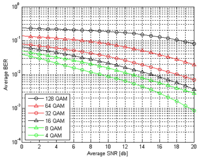
The act of FSO system using the exponentiated gamma channel model with QAM for various values of M (4, 8, 32, 64, 128) is examined. It proves that the performance is best for the lowest values of M. Because as the value of M increases, the error rate is higher and more signal strength is required.

Fig. 3 shows BER vs. SNR of FSO system using 16-QAM for various channel models with a Mach-Zehnder optical modulator. Irradiance is chosen as P = Q = 1 and the turbulence condition is assumed to be strong. The numerical result has been obtained based on values of α and β [25], the BER expression of the gamma channel model, the Rayleigh channel model [26], the gamma-gamma channel model [25], and the proposed exponentiated-gamma channel model (32). Fig. 4 and Fig. 5 show that the proposed exponentiated gamma channel model performs better than existing channel models because, to achieve a BER of 10^-15, the proposed channel model required a signal strength of about 35 dB, whereas it is 43 dB, 58 dB, and more than 60 dB for gamma-gamma, gamma and Rayleigh channel model, respectively. Hence, the proposed channel model enhances the system power gain.

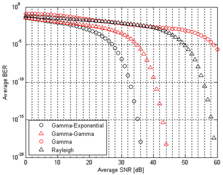
Fig. 3. Comparison of average BER vs. average SNR of FSO system using 16-QAM for various channel models.

Fig. 4 shows BER vs. average SNR of a SISO FSO system with QAM using the exponentiated gamma channel under various values of link distance and refractive index structure parameter. The parameters used in (32) are P = Q = 0.5, σi 2= σj 2= 0.5 and i = j = 1. Fig. 4 indicates that when L = 1000 m and C_n²  = 6 ⸱10^-15 m^-2/3 to achieve a BER of 10^-10 , the required signal strength is 31 dB. But at L = 2000 m and 10^-15 m^-2/3 , the SNR required is 48 dB. That is a gain of about 17 dB is needed to reach a BER of 10^-10 . This shows that the performance of BER is the best under the lowest value of link distance and refractive index structure parameter. This reveals that the link distance has greater effect on the FSO system performance.

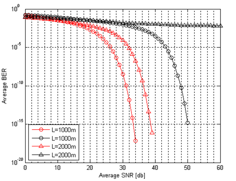
Fig. 4. Average BER vs. average SNR of SISO FSO system with QAM and the exponentiated gamma channel model for different values of link distances.

Fig. 5 presents BER vs. SNR of the SISO and SIMO FSO system with 16-QAM using the exponentiated gamma channel model and Greedy scheduling. The performance is analysed under various link distances, i.e., L = 1000 m and L = 2000 m, C_n²  = 1e−15 m^-2/3 and the irradiance parameter P = Q = 0.5. The numerical results are achieved based on (32) for SISO system and (44) for SIMO FSO system. The performance is better for SIMO with the lowest link distance, i.e., at L = 1000 m. Power gain of about 8 dB is attained by multiple-output system at a BER of 10^-15 using the exponentiated gamma channel model and Greedy scheduling, whereas for a single-output system, the signal strength required is high in order to achieve a BER of 10^-15. With an increase in link distance, BER is more dominant over weak turbulence condition than strong turbulence condition.

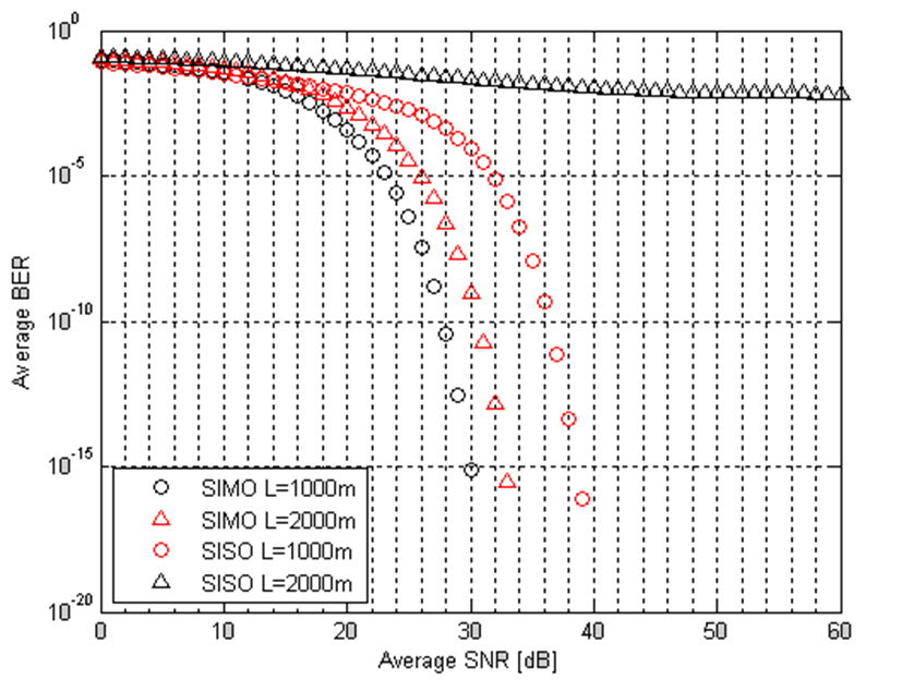
Fig. 5. Average BER vs. average SNR of SISO and SIMO FSO system with QAM and the exponentiated gamma channel model for different values of link distances.

Fig. 6 shows average BER vs. average SNR of FSO system for a single-output and multiple-output FSO system with Greedy scheduling using the exponentiated gamma channel model. BER dependence on SNR is presented considering 16-QAM. The analysis is done with respect to various turbulence conditions (C_n² ), link distance L = 1000 m, and irradiance P = Q = 0.5 The result is depicted based on (32) and (44) for a single output and multiple output, respectively. For C_n²  = 1e−15,with BER as 10^-10 , the signal strength needed is 27 dB and 36 dB, respectively for a multiple output and single output. But for C_n² = 1e−15, the required signal strength for a multiple output and single output is 30 dB and 60 dB, respectively. Hence, it is clear that under strong turbulence conditions, irrespective of the signal at the output, the signal strength needed is higher than under weak turbulence conditions.

Fig. 6. Average BER vs. average SNR of SISO and SIMO FSO system with QAM and the exponentiated gamma channel model for various turbulence conditions.

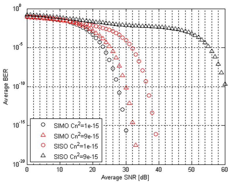
Fig. 7 represents the capacity of the multiple output FSO system with the exponentiated gamma channel model and Greedy scheduling. The result for throughput is achieved based on (36) and (37). Here, the parameters used are νi = 1000, li = 1000 m, pmax = 20. The capacity per-formance is tested and analysed under different turbulence conditions. Fig. 7 indicates that weak turbulence conditions result in higher capacity and strong turbulence conditions result in lower capacity. It clearly shows that capacity of the FSO system mainly depends on turbulence conditions.

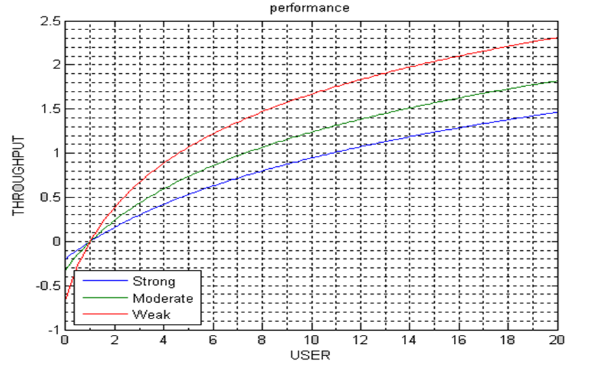
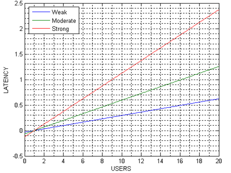
Fig. 7. Average throughput of FSO system with multiple receivers using the exponentiated gamma channel model and Greedy scheduling.

Fig. 8 shows the response of latency for different users of FSO system with the exponentiated gamma channel model and Greedy scheduling under various turbulence conditions. The result shown in Fig. 8 is obtained using (45) with irradiance P = Q = 1, α = 1.3 and β = 0.5. It shows that for weak turbulence conditions, the delay is lower, for moderate turbulence it is slightly higher, and for strong turbulence it is higher. Hence, it is evident that the latency in FSO system depends entirely on turbulence effects.

Fig. 8. Latency of FSO system with multiple receivers using the exponentiated gamma channel model and Greedy scheduling.

Practical sources of fluctuations in FSO systems primarily arise from atmospheric turbulence, temperature gradients, and variations in humidity. These environmental factors cause rapid, random fluctuations in the refractive index of the air, leading to signal degradation such as scintillation and beam wandering, which can significantly affect the optical signal intensity and phase. In addition to turbulence, temporal variations in the air refractive index due to thermal gradients can cause phase shifts, further impacting the stability of the received signal. Aperture averaging is commonly used to mitigate these effects, but it can only partially reduce the turbulence-induced fading. Moreover, rain, fog, and snow can attenuate the optical signal, particularly in the long-wavelength infrared region, which is often used in FSO communication. These practical sources of fluctuation can lead to a higher BER and reduced system reliability. Therefore, any theoretical model must not only account for the turbulence but also consider these real-world phenomena to ensure that the system performs effectively under actual environmental conditions.

The practical impacts of adapting this research are far-reaching, offering solutions to some of the most pressing challenges in FSO communication. By improving BER performance, enhancing system reliability, and enabling deployment in a broader range of environments, the proposed advancements open new possibilities for the widespread adoption of FSO technology. This not only addresses current limitations but also positions FSO systems as a critical component of next-generation communication networks, capable of supporting emerging applications in urban infrastructure, remote connectivity, aerospace, and beyond.

Conclusions

This study presents an advanced FSO communication system using the exponentiated gamma channel model, SC QAM, and Greedy scheduling aiming to enhance system performance in turbulent environments. The analysis reveals that traditional turbulence models, while effective in certain conditions, fail to fully capture the complexities of real-world atmospheric disturbances. By introducing the exponentiated gamma model, this research addresses a critical gap, offering a more flexible and accurate framework for modelling turbulence across a wider range of conditions. The results demonstrate significant improve-ments in BER performance, especially in systems employing multiple receivers in a SIMO configuration. Furthermore, the application of Greedy scheduling enhances the system resilience to turbulence by dynamically optimizing resource allocation based on channel conditions, leading to more efficient communication. While the theoretical analysis provides valuable insights, future work should focus on validating these findings through experimental setups to capture real-world complexities such as beam misalignment, ambient light interference, and dynamic weather conditions. Additionally, the integration of this FSO system with other communication technologies, such as RF or fibre optics, represents a promising avenue for future research to mitigate the limitations of standalone FSO systems and improve overall network robustness. In conclusion, this paper contributes to the growing body of knowledge in FSO communications by proposing an innovative and flexible approach to turbulence modelling, offering practical solutions for optimizing system perfor-mance in diverse environments. The findings open the door for the development of the next-generation optical commu-nication systems that can maintain high-speed data transfer even under challenging atmospheric conditions, paving the way for more reliable and efficient networks in applications ranging from satellite communication to urban connectivity.

Multiple-output free space optical system with exponentiated gamma channel model and Greedy scheduling

Article Info

Abstract