Computer-generated holography is a technology valuable for efficient projection and three-dimensional displays, with a growing number of calculation algorithms and relatively simple optical setups for image reconstruction. Among available technologies, liquid crystal on silicon spatial light modulators can provide uncomplicated phase modulation of incident wavefronts. However, these devices face challenges to overcome, such as the presence of multiple image duplicates in hologram reconstructions. Here, we propose a method for reducing visibility of those duplicates in which the volume and complexity of the setup remain the same. It is based on randomisation of positions of light-modulating pixels and distorting the otherwise regular pixel array of the modulator, without modifying the device. We present a theoretical analysis and results obtained in both simulations and experiment. Signal-to-noise ratio in the areas surrounding the desired image is shown to decrease, suppressing the presence of image duplicates. Various levels of randomisation are considered and can be selected with specific applications in mind.

Introduction

Holography – the art of recording the information about both intensity and phase of the wavefront, as well as its reconstruction – has been present in scientific studies since 1948 when Gabor introduced the idea [1]. Since then, the development of technology enabled various applications of this phenomenon, from static, analogue and digital holography for medicine, 3D imaging, holographic TV and compressive holographic tomography [2–4], to computer-generated holography for beam conversion, 3D displays [5–7] and dynamic holographic projection [8]. However, despite the many benefits of this technology and the progressing miniaturisation of setups, some challenges remain. The most widely used devices for displaying numerically calculated holograms, called spatial light modulators (SLMs), are digital micromirror devices (DMDs) applicable for amplitude holograms and liquid crystal on silicon (LCoS) SLMs that offer phase modulation of grey-scale values. In LCoS SLMs, which are the focus of our research, the fixed pixel array causes the presence of wavefront duplicates in the reconstructed far field [9]. Those duplicates can be removed, for example, by employing 4f systems for spatial filtering [10, 11], which, however, leads to an increased volume of more complex projection setups and hinders miniaturisation. It is a known challenge in holography and has been addressed in Fresnel holography by altering algorithms that calculate phase patterns [12], or in near-field point-formed holograms by adding a diffusive element [13]. In dynamic Fourier holography, this effect is just as important to address [14, 15]. However, the state-of-the-art does not offer an efficient, low-volume solution for this type of holography. One of the considered approaches is focused on devices of different builds, which can limit the visibility of ghost images. For example, Smalley et al. presented a leaky-mode approach [16]; other previously published works introduce a new ultrafast material for holographic recording [17, 18]. However, such devices are often difficult to control or exhibit a highly decreased efficiency, which is why a solution for easy-to-use LCoS SLMs would be favourable.

The problem of limiting the number of visible diffraction orders can also be encountered in other fields of diffractive optics, i.e., diffraction gratings, with various proposed solutions. Simple amplitude sinusoidal gratings are efficient in limiting diffraction orders to only three central diffraction orders [19], however, smooth sinusoidal gratings are not possible to display on LCoS SLMs and more complex solutions need to be considered [20].

Research on structures with disrupted regularity of their patterns has been reported to reduce the number of visible duplicates, e.g., for zig-zag gratings [21], grooves of randomised positions [22, 23], or even and odd rows of elementary cells shifted in relation to each other [24]. For computer-generated phase-only holograms, which are 2D distributions of phase shift values, the most relevant findings seem to refer to the randomized positioning of each elementary cell of a 2D grating [25], as researched by Wei et al. [9], who investigated its application for static diffractive structures. When a random shift was applied to the pixels of a manufactured structure, the visibility of duplicated images was reduced at the cost of increased noise.

In our work, we discuss a randomisation method for reducing the visibility of image duplicates that can be applied specifically for LCoS SLMs of static, periodic pixel patterns. In this process, the formation of the replicas of images is suppressed and the intensity in the area surrounding the main target image is redirected into static noise instead. We introduce a theoretical analysis of the method, compare different levels of randomisation, and present experimental results.

Theoretical discussion and simulations

LCoS SLMs consist of fixed arrays of electrodes. As such, it is not possible to simply change the pixels positions to introduce randomisation. Afuture usage could use a subpixel mask, covering the edges of each pixel in an adjustable way, without sacrificing the bandwidth of the SLM. However, for some chosen applications, as well as in general proof of concept, randomisation can be introduced to these devices by undersampling, as follows: A phase hologram can be resized, e.g., stretched four times in both directions, so that each phase value corresponds to 4 × 4 pixels. We can then divide an SLM into such 4 × 4 px subsections and randomly choose only one pixel within its area, which will display the phase-shift value defined by the stretched hologram.

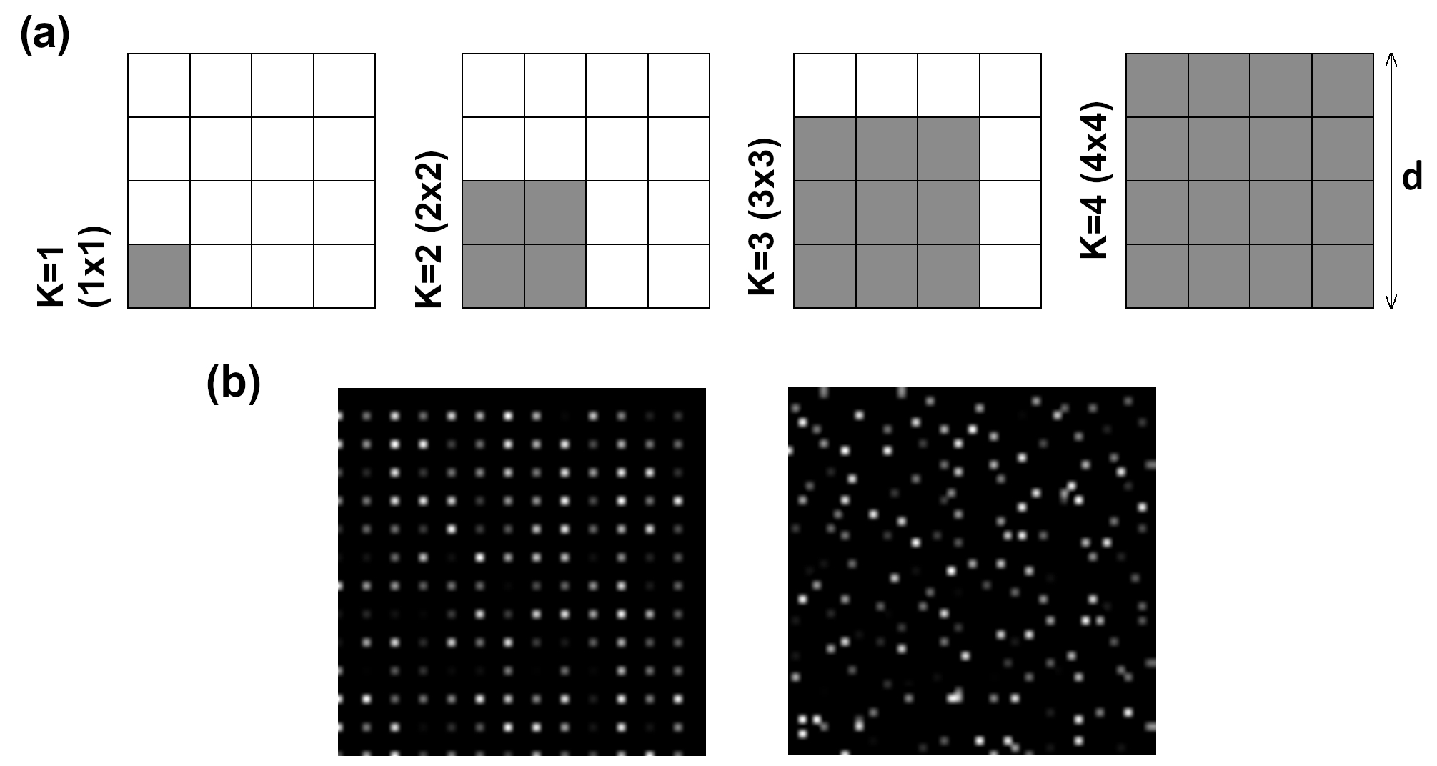
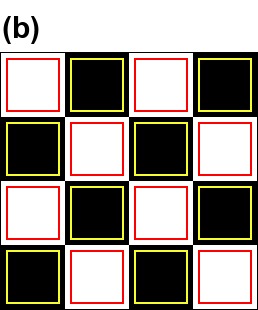
In such an SLM subsection, four possible randomisation levels can be considered, as shown in Fig. 1(a): none, low, medium, and high. A visual example of a resulting randomised hologram can be seen in Fig. 1(b).

‌

**Fig. 1.**Pixel positions with applied randomisation. (a) Levels of randomisation for a 4 × 4 subsection of an SLM; from left to right: none, low, medium, and high level. Grey areas correspond to possible positions of the single active pixel. (b) Exemplary pixel patterns to be displayed on an LCoS SLM: no randomisation (left) and high randomisation level (right).

Theoretical analysis of the proposed randomisation follows similar principles as in the work by Wei et al. [9] with an important difference that in the case of LCoS SLMs, the positioning of pixels is discrete rather than continuous. Let us assume a periodic pattern of SLM subsections, comprised of 4 × 4 SLM pixels each. These subsections form elementary cells of this pattern, with a period 𝑑, equal to the width of the SLM subsection. Each elementary cell consists of an array of 𝐾 × 𝐾 pixels [𝐾 = 1, 2, 3, 4, see: grey areas in Fig. 1(a)], each with a side of 𝑑/4. For easier analysis, within each such cell, only one randomly chosen pixel is transparent and the others are black (see section 3 for further discussion). The coordinates of the centre of each such pixel can be written as (𝑛𝑑 + 𝜉_𝑛𝑚, 𝑚𝑑 + 𝜂_𝑛𝑚), where 𝑛 ∈ (−𝐿, ...0, ...𝐿) and 𝑚 ∈ (−𝐻, ...0, ...𝐻), and 𝜉 and 𝜂 are randomisation factors. The transmittance of an array of 𝑁 = 2𝐿 + 1 by 𝑀 = 2𝐻 + 1 pixels (𝐿, 𝐻 ∈ N) can be described in relation to coordinates in the SLM plane (𝑢, 𝑣) as:

\( t(u, v)=\sum_n \sum_m \operatorname{rect}\left(\frac{u-n d-\xi_{n m}}{d / 4}\right) \operatorname{rect}\left(\frac{v-m d-\eta_{n m}}{d / 4}\right) \) (1)

If we illuminate this pattern with a plane wave, we can calculate the diffraction far field as a Fourier transform ℱ(𝜈_𝑥, 𝜈_𝑦), where 𝜈_𝑥 and 𝜈_𝑦 are related to the coordinates in the diffraction field. Up to an insignificant factor, the intensity distribution in the far-field can then be written as follows:

\( \begin{aligned} I\left(v_x, v_y\right)= & \mathscr{F}\left(v_x, v_y\right) \mathscr{F}^*\left(v_x, v_y\right) \\ = & \left(\frac{d^2}{4^2}\right)^2 \operatorname{sinc}^2\left(\frac{v_x d}{4}\right) \operatorname{sinc}^2\left(\frac{v_y d}{4}\right) \\ \sum_n \sum_m & \times \sum_{n^{\prime}} \sum_{m^{\prime}} e^{i 2 \pi v_x\left(n^{\prime}-n\right) d} e^{i 2 \pi v_y\left(m^{\prime}-m\right) d} \\ & \times e^{i 2 \pi v_x\left(\xi_{n^{\prime} m^{\prime}}-\xi_{n m}\right)} e^{i 2 \pi v_y\left(\eta_{n^{\prime} m^{\prime}}-\eta_{n m}\right)} \end{aligned} \) (2)

\( \begin{aligned} & I\left(v_x, v_y\right)=A \times\{N \times M \\ & \quad+\sum_n \sum_m e^{-i 2 \pi v_x n d} e^{-i 2 \pi v_y m d} \\ & \quad \times \sum \sum\left(n^{\prime}, m^{\prime}\right) \neq(n, m) e^{i 2 \pi v_x n^{\prime} d} e^{i 2 \pi v_y m^{\prime} d} \\ & \left.\quad \times E_{\text {val }}\left[e^{i 2 \pi v_x\left(\xi_{n^{\prime} m^{\prime}}-\xi_{n m}\right)} e^{i 2 \pi v_y\left(\eta_{n^{\prime} m^{\prime}}-\eta_{n m}\right)}\right]\right\} \end{aligned} \) (3)

where 𝐸_𝑣𝑎𝑙 is the expected value, that is the constant average value of the expression. The second sum can be rewritten as a subtraction of a sum for (𝑛′, 𝑚′) = (𝑛, 𝑚) from the sum of all factors. The sum of all factors can in turn be obtained as the product of sums of a geometric sequence, for both the first and the second sum of (3):

\( \begin{aligned} \sum_{n^{\prime}} \sum_{m^{\prime}} & e^{-i 2 \pi v_x n^{\prime} d} e^{-i 2 \pi v_y m^{\prime} d} \\ & =\sum_{n^{\prime}=-L}^L \sum_{m^{\prime}=-H}^H e^{-i 2 \pi v_x n^{\prime} d} e^{-i 2 \pi v_y m^{\prime} d} \\ & =\frac{\sin \left(\pi v_x d N\right)}{\sin \left(\pi v_x d\right)} \frac{\sin \left(\pi v_y d M\right)}{\sin \left(\pi v_y d\right)} \end{aligned} \) (4)

\( \begin{aligned} & I\left(v_x, v_y\right)=A \times\{N \times M \\ & +E_{v a l}\left[e^{i 2 \pi v_x\left(\xi_{n^{\prime} m^{\prime}}-\xi_{n m}\right)} e^{i 2 \pi v_y\left(\eta_{n^{\prime} m^{\prime}}-\eta_{n m}\right)}\right] \\ & \left.\quad \times\left[\frac{\sin ^2\left(\pi v_x d N\right)}{\sin ^2\left(\pi v_x d\right)} \frac{\sin ^2\left(\pi v_y d M\right)}{\sin ^2\left(\pi v_y d\right)}-N \times M\right]\right\} \end{aligned} \) (5)

In the considered case, the centres of active pixels of 𝐾 × 𝐾 arrays are positioned at discrete 𝜉_𝑛𝑚, 𝜉_{𝑛′𝑚′} , 𝜂_𝑛𝑚, 𝜂𝑛′𝑚′ , which can each take one of 𝐾 discrete values:

\( \xi_j=\frac{d}{4} j, \quad \eta_j=\6rac{d}{4} j, \quad j=0,1, \ldots K-1 \) (6)

The expected value 𝐸_𝑣𝑎𝑙 considers all 𝐾4 variations with repetitions for all possible 𝜉_𝑛𝑚, 𝜉_{𝑛′𝑚′} , 𝜂_𝑛𝑚, 𝜂𝑛′𝑚′ for elementary cells (𝑛′, 𝑚′) ≠ (𝑛, 𝑚):

\( \begin{aligned} E_{v a l}\left[e^{i 2 \pi v_x\left(\xi_{n^{\prime} m^{\prime}}-\xi_{n m}\right)} e^{i 2 \pi v_y\left(\eta_{n^{\prime} m^{\prime}}-\eta_{n m}\right)}\right] & \\ = & \frac{1}{K^4}\left[\sum_{j=0}^{K-1} \sum_{k=0}^{K-1} e^{i 2 \pi\left(v_x \xi_j+v_y \eta_k\right)}\right] \\ & \times\left[\sum_{j=0}^{K-1} \sum_{k=0}^{K-1} e^{i 2 \pi\left(v_x \xi_j+v_y \eta_k\right)}\right]^* \\ = & \frac{1}{K^4}\left|\sum_{j=0}^{K-1} \sum_{k=0}^{K-1} e^{i 2 \pi\left(v_x \xi_j+v_y \eta_k\right)}\right|^2 \\ = & \frac{1}{K^2}\left|\sum_{j=0}^{K-1} e^{i 2 \pi v_x \xi_j}\right|^2 \times \frac{1}{K^2}\left|\sum_{k=0}^{K-1} e^{i 2 \pi v_y \eta_k}\right|^2 \end{aligned} \) (7)

We introduce notations 𝑥 = 𝜈_𝑥𝑑 and 𝑦 = 𝜈_𝑦𝑑 for positions in the diffraction field plane with respect to diffraction orders: 𝜈_𝑥 = 𝑝/𝑑, 𝜈_𝑦 = 𝑞/𝑑; 𝑝, 𝑞 ∈ Z. Then, for example, (𝑥 = 1, 𝑦 = 0) corresponds to the first diffraction order in the horizontal direction, and (𝑥 = 1/2, 𝑦 = 0) to the middle point between the zeroth and first horizontal diffraction orders. The expected value can thus be rewritten as:

\( \begin{aligned} & E_{v a l}\left[e^{i 2 \pi v_x\left(\xi_{n^{\prime} m^{\prime}}-\xi_{n m}\right)} e^{i 2 \pi v_y\left(\eta_{n^{\prime} m^{\prime}}-\eta_{n m}\right)}\right]=g(x) g(y), \\ & \text { where } g(x)=\frac{1}{K^2}\left|\sum_{k=0}^{K-1} e^{i \pi x k / 2}\right|^2 . \end{aligned} \) (8)

For 𝐾 = 1, that is, for a nonrandomised pixel pattern, 𝑔(𝑥) = 1. For other randomisation levels:

\( \begin{array}{rr} K=2: & g(x)=\frac{1}{2}\left[1+\cos \left(\frac{\pi x}{2}\right)\right] \\ K=3: & g(x)=\frac{1}{9}\left[3+4 \cos \left(\frac{\pi x}{2}\right)+2 \cos (\pi x)\right] \\ K=4: & g(x)=\frac{1}{16}\left[4+6 \cos \left(\frac{\pi x}{2}\right)+4 \cos (\pi x)\right. \\ & \left.+2 \cos \left(\frac{3 \pi x}{2}\right)\right] \end{array} \) (9)

With this in mind, we can rewrite (3) as a relation of intensity 𝐼 and coordinates in the diffraction field (𝑥, 𝑦):

\( \begin{aligned} & I(x, y)=I_1(x, y)+I_2(x, y) \\ &=\left(\frac{d}{4}\right)^4 \operatorname{sinc}^2\left(\frac{x}{4}\right) \operatorname{sinc}^2\left(\frac{y}{4}\right)\{N \times M \\ &\left.+g(x) g(y)\left[\frac{\sin ^2(\pi N x)}{\sin ^2(\pi x)} \frac{\sin ^2(\pi M y)}{\sin ^2(\pi y)}-N \times M\right]\right\} \end{aligned} \) (10)

\( \begin{aligned} I_1(x, y)= & \left(\frac{d}{4}\right)^4 \operatorname{sinc}^2\left(\frac{x}{4}\right) \operatorname{sinc}^2\left(\frac{y}{4}\right) \\ & g(x) g(y) \frac{\sin ^2(\pi N x) \sin ^2(\pi M y)}{\sin ^2(\pi x)} \sin ^2(\pi y) \end{aligned} \) (11)

\( \begin{aligned} I_2(x, y)= & \left(\frac{d}{4}\right)^4 \operatorname{sinc}^2\left(\frac{x}{4}\right) \operatorname{sinc}^2\left(\frac{y}{4}\right) \\ & (N \times M)[1-g(x) g(y)] \end{aligned} \) (12)

𝐼1 (𝑥, 𝑦) describes the useful signal with the diffraction orders resulting from the pixel pattern. The geometry of intensity peaks in diffraction on a comb grating is modulated by the product of intensity distribution of a single pixel and the expected value:

\( \mathcal{M}(x, y)=\operatorname{sinc}^2\left(\frac{x}{4}\right) \operatorname{sinc}^2\left(\frac{y}{4}\right) g(x) g(y) \) (13)

We can interpret 𝐼2 (𝑥, 𝑦) as continuous noise, present only for randomised pixel patterns, with intensity modulated by:

\( \mathcal{R}(x, y)=\operatorname{sinc}^2\left(\frac{x}{4}\right) \operatorname{sinc}^2\left(\frac{y}{4}\right)[1-g(x) g(y)] \) (14)

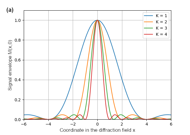
Images reconstructed from holograms have non-negligible dimensions. For this reason, it is important to consider not just discrete values, but the envelopes of M(𝑥, 𝑦). Figure 2(a) shows the distribution M(𝑥, 0) in the horizontal direction (analysis of the vertical direction would be analogous). Not only do certain diffraction orders correspond to zero or near-zero intensities, but the areas around them are visibly suppressed as well.

The noise distribution in the horizontal direction can be calculated from R(𝑥, 0), as presented in Fig. 2(b). In the centre of the field, the noise is minimal, reaching its maximal value between the centre of the field and the second order of diffraction, closer to the centre for higher values of 𝐾. Randomisation of pixel positions leads to increased noise within the areas of higher diffraction orders, and as such, lowers the visibility of duplicated images, already suppressed by the altered M(𝑥, 𝑦) envelope. It is expected that for a properly chosen randomisation level, those undesired duplicates will be concealed by the noise, while the central image will remain relatively undistorted.

‌

Fig. 2. Theoretical distributions calculated for periodic and randomised pixel patterns as a function of diffraction orders. (a) Signal envelopesM(𝑥, 0); (b) noise distributions R(𝑥, 0) in which the blue line overlaps with the horizontal axis.

This randomisation effect, despite the increased noise levels, can be highly beneficial for certain applications, such as dynamic holographic projection, in which additional moving images would be unacceptable to viewers, while the limited, static noise would be less disruptive. Another example of a field where the presented image suppression would be favourable is laser-beam manufacturing or ablation, in which the interaction between light and the material occurs above a certain threshold. In such a case, low-intensity noise will not affect the process, whereas a pattern replica of high intensity would.

Signal-to-noise ratio (𝑆𝑁𝑅𝑡ℎ) of the whole intensity distribution can be defined as the ratio of intensity integrals of the reconstructed signal 𝐼1 (𝑥, 𝑦) and the background noise 𝐼2 (𝑥, 𝑦):

For a subsection of 4 × 4 pixels, theoretical 𝑆𝑁𝑅𝑡ℎ values of: 13 for 𝐾 = 2, 18 for 𝐾 = 3, and 1 15 for 𝐾 = 4 are obtained. The values show that the fraction of incident intensity that forms the images decreases rapidly with increasing levels of randomisation. This means that the randomisation method might have limitations in certain applications, and different levels of randomisation might be appropriate for images displayed in the centre of the field and for those spanning the whole area of a single image reconstruction. To test the proposed method on a specific case of hologram reconstruction, the phase hologram of a chequered pattern (containing 16 black and white squares) was calculated using the IFTA algorithm [26, 27] on a 512 × 512 px calculation array. This phase distribution was then oversampled in such a way that a single phase-shift value corresponded to a whole 4×4 subsection of the 2048×2048 array, and only one pixel within this subsection displayed phase information. The oversampled holograms were reconstructed using the fast Fourier transform. 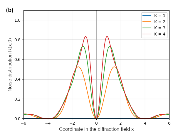From the resulting complex distribution, intensity was calculated as the square value of the complex amplitude. The obtained image reconstructions (Fig. 3) show the suppression of image duplicates in higher diffraction orders for higher randomisation levels, as predicted by the presented theoretical analysis. The increase in background noise is also visible. A sufficiently high randomisation level can lead to suppression of image duplicates even in the area of the second diffraction order, by adjusting both the signal envelope and the noise outweighing the undesired signal.

‌

Fig. 3.(a) Simulated image reconstructions: normalised intensity distributions (here with gamma = 1.5 for readability in print) with their horizontal cross-sections along the marked yellow line. Area of a single target image is marked with a blue square. From left to right and top to bottom: no pixel randomisation, low, medium, high randomisation level. (b) Areas of the chequered pattern, bright (marked in red) and dark (marked in yellow), used for SNR calculations.

\( S N R=\frac{\iint I_{\text {bright }}(x, y) d S-\iint I_{\text {dark }}(x, y) d S}{\iint I_{\text {dark }}(x, y) d S} \) (16)

For this approach, the SNR will assume values above 0 when the image intensity is higher than the noise. Calculations were carried out for the whole image (all 16 squares) and the centre of the image area (central 4 squares) to consider the applicability of the solution for images of both large and small angular size. The eight nearest duplicates surrounding the main desired image, all visible in Fig. 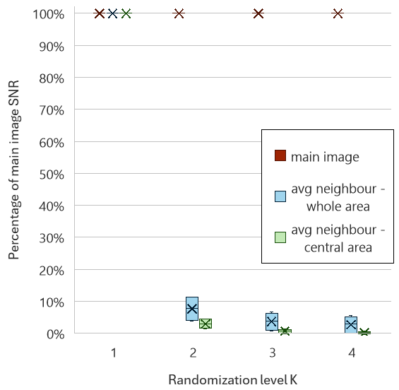3(a), are considered neighbouring images, for which an averaged value of SNR was calculated for a more straightforward comparison. Fig. 4 (a box plot showing distribution of data into quartiles, with mean value marked with an x) shows comparison of SNR values within the main image and its neighbouring image duplicates. The visibility of undesired images in comparison to the central area of the image is successfully reduced.

‌

Fig. 4.Simulation results. Box plot: comparison of the SNR within the main image and the averaged neighbouring image duplicates for all randomisation levels, as a percentage of main image SNR.

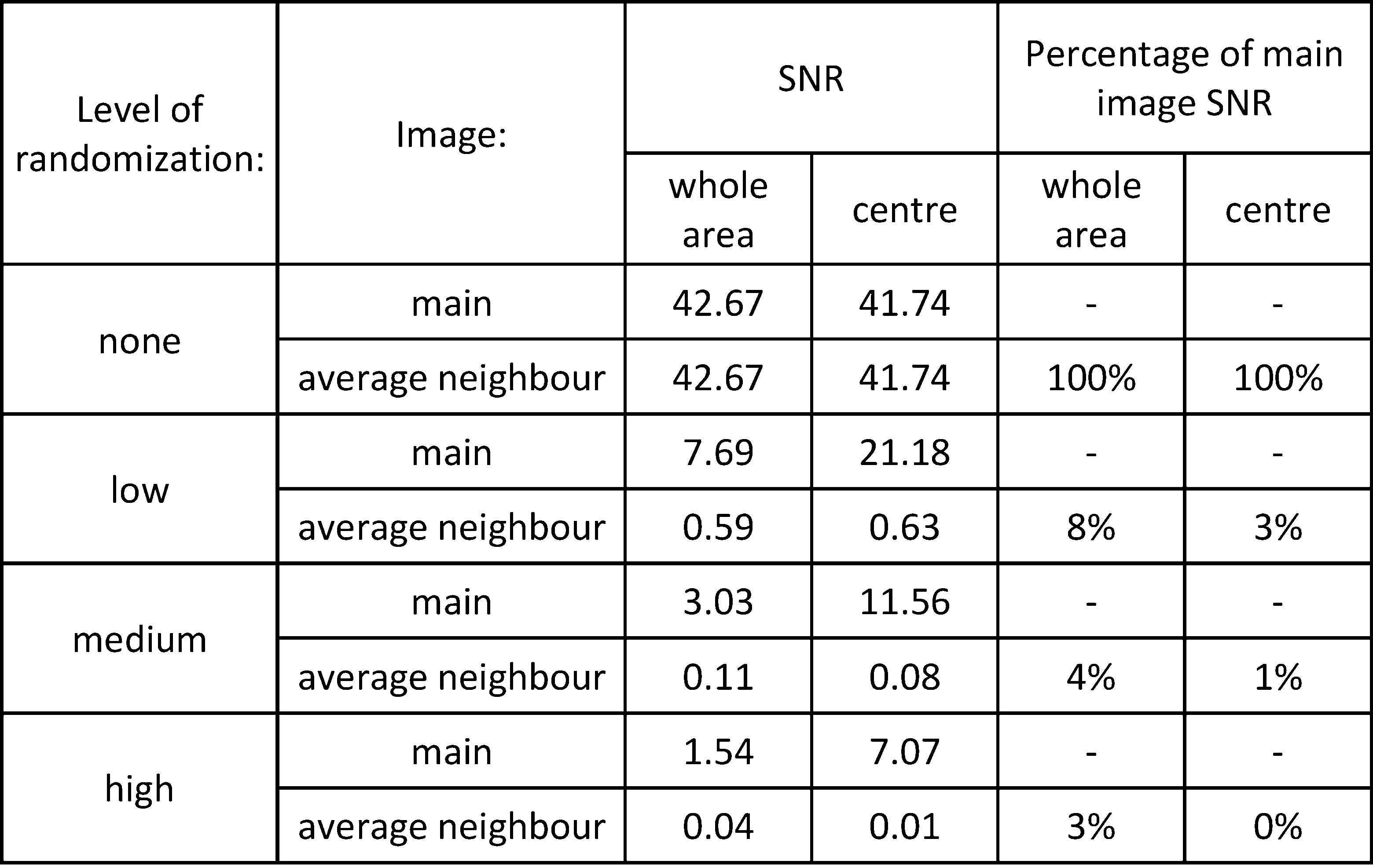
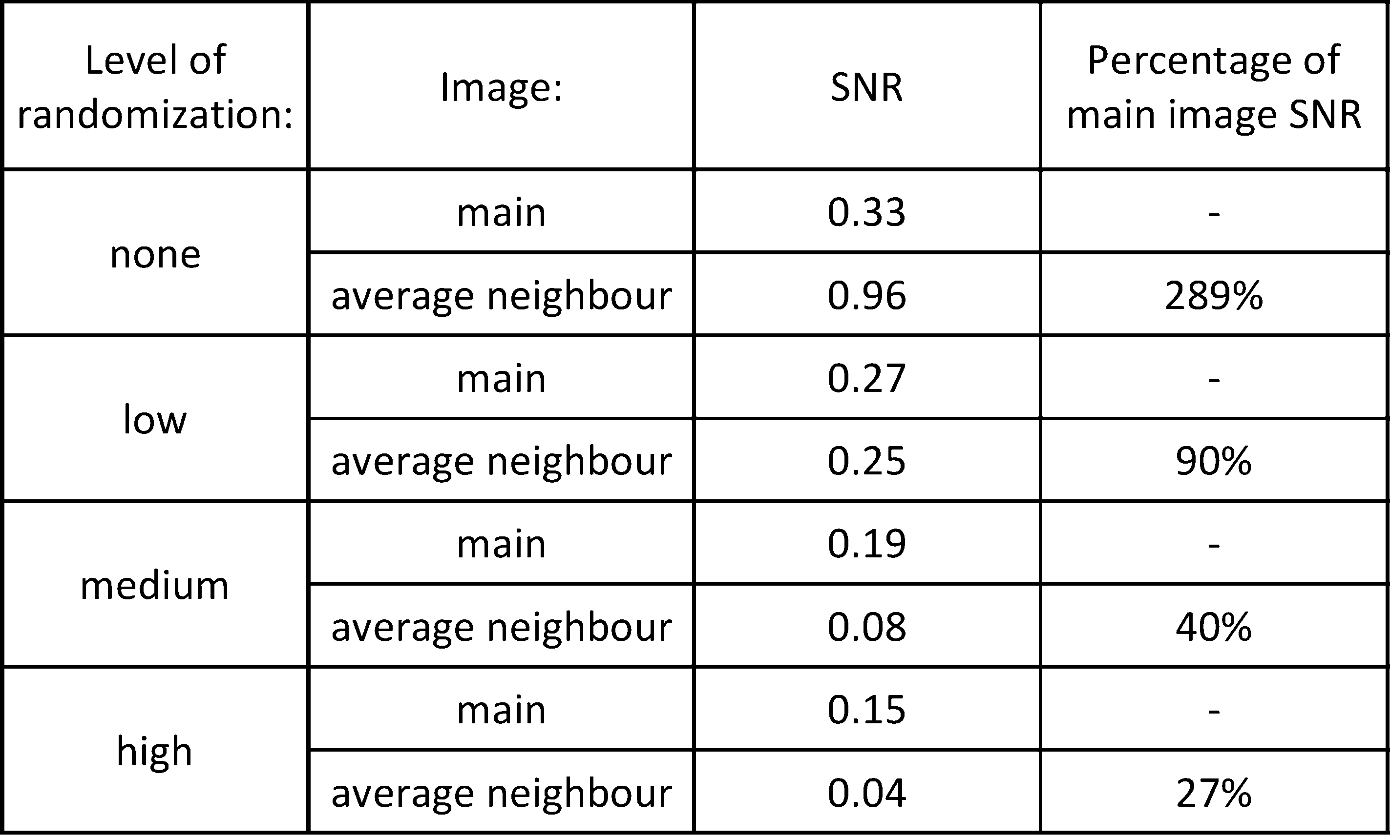
Table 1 presents the values of 𝑆𝑁𝑅 for various levels of randomisation for further numerical analysis. In line with theoretical expectations, the SNR declines for all images when randomisation introduces noise to the hologram reconstruction. However, it is worth noting that the SNR for the main image decreases slower than for the image duplicates. The initial SNR value of 42.67 in the main image area for no randomisation drops to 7% of its value (to 3.03) when medium randomisation is applied, while the value of 42.67 for the neighbouring images drops to a much lower 0.11 (less than 1%). For the high randomisation level, the neighbouring duplicates are similarly indistinguishable from the background noise, with an SNR equal to 0.04, while the main image is still visible (SNR of 1.54). For images spanning the whole area of a single diffraction order, this strongest randomisation effect might, in some applications, cause too much noise presence. However, if the analysis is focused on the central area, where the presumably most relevant information is displayed and where the images of a smaller size are typically positioned, the advantage of the proposed method is even more visible. For example, for low randomisation level, the central SNR in the main image decreases only by half, while in the neighbouring areas, the central SNR drops by 98% (to 0.63). This means that for images of smaller angular size, pixel randomisation is even more beneficial, as could be seen in previously published limited premilinary results [17].

Experimental validation

The holograms used in the simulations were then prepared for experimental validation. In theoretical analysis, it was possible to assume that pixels not carrying phase information are not transparent and do not contribute to the resultant intensity distribution. However, in the case of a real LCoS SLM, those inactive pixels not only cannot produce 0 values of amplitude and will instead act as a mirror for the incident light, but also might carry a phase value influenced by the neighbouring active pixels. This leads to the presence of a central bright spot in the image reconstruction. To reduce its intensity and improve the diffraction efficiency of the SLM device, a half-wave plate was used in our setup to adjust the polarisation of the incident beam. The central noise can be further suppressed with additional methods. In our experiment, phase values of those inactive pixels were set as 0 and 𝜋, alternately, in a method researched by Shimobaba et al. [28]. Two resulting wavefronts modulated by these two values, respectively, should interfere destructively and reduce the influence of undiffracted light on the hologram reconstruction. However, the experiment shows the presence of other potential distortions of the image.

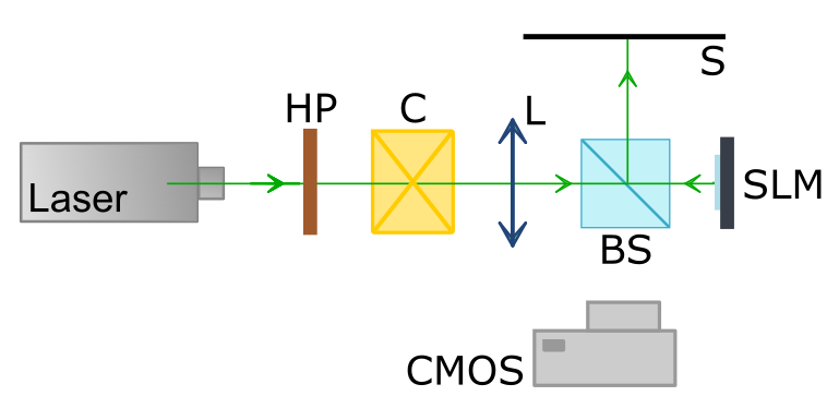
An experimental setup was built as described in the schematic in Fig. 5. Since the intensity distribution at the focal length of the lens corresponds to the intensity obtained through a Fourier transform of a wavefront [19], the presented setup leads to a reconstruction of a Fourier hologram on the screen placed at the focal length of the lens. The modulator used was HOLOEYE PLUTO of 8.0 𝜇m pixel size, 93% fill factor, and FHD resolution. It was illuminated with a laser beam of wavelength 𝜆 = 532 nm. The beam splitter was placed 16 cm from the focusing lens and 4 cm from the SLM, and the distance from the beam splitter to the screen was 140 cm. The reconstruction of the holograms displayed on the SLM was observed on a screen and photographed using a CMOS camera. 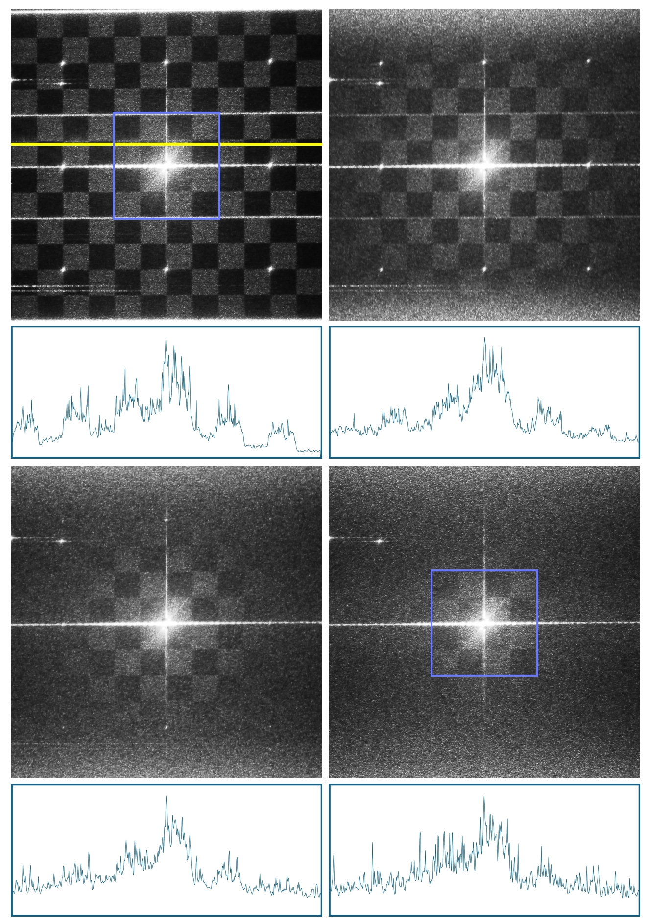Images for various levels of randomisation are presented in Fig. 6. The visible noise aligns with theoretical assumptions, though it is more pronounced than in simulations because of imperfections of the experimental setup, such as distortions of the displayed phase caused by pixel crosstalk. However, creating the optimal hologram reconstruction setup was not the goal of this research and the obtained results are more than sufficient to observe the discussed phenomenon.

‌

**Fig. 5.**Schematic of a setup for hologram reconstruction. Laser source of 𝜆 = 532 nm, SLM – LCoS SLM HOLOEYE PLUTO, HP – half-wave plate, C – collimator, L – lens focusing the wavefront on S – screen, BS – beam splitter, CMOS - camera.

‌

**Fig. 6.**Image reconstruction from randomised holograms on an undersampled SLM with their normalised horizontal crosssections along the marked yellow line. Area of a single target image is marked with a blue square. From left to right and top to bottom: no pixel randomisation, low, medium, and high randomisation level.

To confirmthe qualitative results, a numerical analysiswas also performed. SNR was calculated according to (16) for images obtained for all randomisation levels. The calculations were carried out only for the full image area (16 black-andwhite squares) this time, as the high central noise in the experiment would strongly impact the results for a smaller, limited area which was considered in simulation results. As presented in Fig. 7 and Table 2, the SNR of neighbouring image duplicates decreases with increasing randomisation levels, confirming the effect predicted by theoretical analysis and simulations. For the highest level of randomization, the SNR value decreases by 55% within the main image and by 96% in the surrounding image duplicates. This difference leads to the lack of distinguishable replicas in hologram reconstruction. Although the effect seems weaker than in the simulations, this can be linked to strong presence of the undiffracted light in the experiment, which lowers the initial SNR of the main image: with no randomisation applied, the SNR of the neighbouring images was almost three times higher than the SNR within the target image (0.96 compared to 0.33). After applying the highest randomisation, the SNR of image duplicates reaches a value as low as 27% of the main image SNR, which is a relevant improvement.

‌

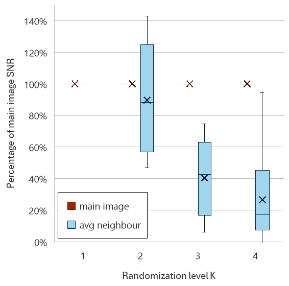
**Fig. 7.**Experimental results. Box plot: comparison of the SNR within the main image and the averaged neighbouring image duplicates for all randomisation levels, as a percentage of main image SNR. Neighbouring images for the case of no randomisation far exceed the SNR of the main image, and are not visible in the chart.

Conclusions

The presented method is successful in reducing the visibility of duplicate images in a holographic reconstruction of dynamic Fourier holograms. We achieved the visual limitation of distinguishable images to the centre of the display field and carried out the numerical analysis of obtained simulation and experimental data that confirm the subjective visual evaluation of this effect. While noise increases and the SNR of all images is lower compared to the case of no randomisation, the ratio of SNR between the neighboring duplicates and the main desired image decreases. The numerical analysis (see Table 1) shows that for the highest level of randomisation considered, this ratio is as low as 3%. This solution can be applied in a holographic projection, e.g., in efficient, miniaturised projectors or head-up displays, which demand low volume of a setup and in which noise distribution that does not shift depending on the displayed image is a lesser disruption than multiple replicas of the desired image. It could also be beneficial for applications with threshold effects, e.g., in laser-beam fabrication, where low-intensity noise does not impact the outcome. Importantly, the level of randomisation can be chosen based on a particular application and target size of the reconstructed pattern. Further research into the optimal size of the SLM subsection is needed, as only 4 × 4 areas have been analysed so far.

Authors’ statement

Research concept and design, J.S. and A.K.; collection and/or assembly of data, J.S., J.B., K.K. and K.P.; data analysis and interpretation, J.S., J.B. and K.K.; writing the article, J.S.; critical revision of the article, K.P. and A.K.; final approval of article, J.S. and A.K.

Acknowledgements

This research was funded by the National Science Centre, Poland under the Preludium program (021/41/N/ST7/01520), and by the National Center for Research and Development, Poland under the LIDER program (LIDER/15/0061/L- 9/17/NCBR/2018).

Randomisation of undersampled pixels for image duplicate suppression in holographic projection

Article Info